Generative Art

Howdy everybody! 

So this posting is a bit different from my other ones which have mostly had to do with graphs. It was in an information visualization class I'm taking that we were recently asked to create our own generative art (programs to produce artsy stuff). For my project I decided to write up some javascript code to generate Mondrian inspired art. I had always thought that his art looked like something that could be created through code, and my intuition was right. What you see below is the result of my programming labors. Every time that you click the Generate Mondrian button you get a new randomly generated Mondrian's Broadway inspired work of art. Refreshing the web page will also give you a new result. Pretty cool huh? ;D  

So how did I do it? Well, to be quite frank I didn't use any fancy algorithms in the process. My code basically involves randomly generating rectangles within an html5 canvas. The number of thin yellow rectangles/columns running from top to bottom was randomly chosen to be a number within a certain range. The same applied to the number of yellow rectangles/rows spanning the canvas from left to right. The number of small grey, red or blue squares to be drawn on each yellow rectangle was also random (constrained by upper and lower bounds as well). To make sure that the yellow rectangles did not line up together and produce thick rectangles, I only drew a rectangle on the canvas if its x or y coordinates were equal to some number modulo 2 (i.e. I made sure that there was some spacing between yellow rows and columns). The final touch was randomly generating some larger red or blue rectangles to layer on top of the rest of the canvas art. I chose a brighter color of red than Mondrian's original brick red for this final part. I thought that the generated art popped out more with this revised shade of red. If you would like to save a copy of any of the randomly generated Mondrians just right click on the image and follow the standard save image as procedure.  

P.S. If you'd like to see more artsy stuff then I'd recommend that you check out my other blog: Joys of a Craftista 
http://craftistajoys.blogspot.com/



Generate Mondrian

Practice

Strongly Regular Graphs

So the post before last I wrote a summary of my summer RMMC trip to Wyoming. As readers of that post will know, the summer topic selected for that annual conference was algebraic graph theory. Many, many, MANY things were discussed there, so many that to write about all of them would be an unrealistic endeavor. It would be a shame not to mention at least one topic from the conference though, so today I will be discussing a particular class of graphs that turned up in several of the contributed RMMC talks: strongly regular graphs. 

Those with some acquaintance with graph theory have most likely heard of regular graphs at the least. Those are the simple graphs (no loops nor multiple edges) where all of the vertices have the same nonnegative degree k. Examples of this include the empty graph (just includes a bunch of isolated points) of regular degree 0, the complete graph of regular degree n-1 (assuming n is the number of vertices in said graph), the Petersen graph (imagine what the drawing of the cocky looking guy above would look like if we only included the black dots and lines between dots) of regular degree 3, simple cycles which are regular of degree 2, and so on. 

The focus of this posting is on undirected graphs, but for the sake of completeness it should also be noted that the notion of regularity can also be extended to directed graphs or digraphs. In this case saying that a digraph is regular means that the indegree of each vertex in the graph equals its outdegree. A very simple example of a regular directed graph is a cycle that has had its edges oriented clockwise or counterclockwise. 

With some basic notion of graph regularity we can know move on to the main post topic: strong graph regularity. When I hear strong regularity, I immediately think the implication is that a graph with such a property is regular in many ways, and this turns out to be true. In order to define a strongly regular graph a total of four parameters must be specified: n, k, lambda, and u. n is the number of vertices in the graph, k the degree of all vertices (i.e. strongly regular graphs are regular as defined previously), lambda is the number of common neighbors that every pair of adjacent vertices in the graph share, and u is the number of common neighbors that any two non-adjacent vertices of the graph share. Like many things in graph theory, the way to understand this is through visual example, so consider the Petersen graph. It has a total of n = 10 vertices and is regular of degree 3. A quick inspection of the graph should reveal that any two adjacent vertices share no common neighbors (implying that the graph is triangle free) and any two nonadjacent vertices have exactly one neighbor in common. By the above definition then we can classify the Petersen graph as a strongly regular ones with parameters 10, 3, 0 and 1 respectively. This is often expressed more compactly by saying that the Petersen graph is srg(10, 3, 0, 1). 

So what makes strongly regular graphs so special besides their satisfaction of numerous regularity conditions? Well for one they have some interesting algebraic properties. If one was to calculate the eigenvalues of a strongly regular graph, it would be found to have exactly three distinct ones. Even more so, these eigenvalues can be expressed in terms of the parameters n, k, lambda and u. The complete derivation involves a few clever observations and careful tinkering with some equations. 

The first eigenvalue is not hard to figure out. Because a strongly regular graph is regular of degree k, it must have k as an eigenvalue. The way to see this is by looking at the multiplication of the graph's adjacency matrix A with the all one's eigenvector. Since each row of A has k ones, multiplying the two will result in entries of k in the resulting vector (i.e. k times the original all one's vector). 

Now, how about the remaining eigenvalues? To find them we have to make a few key observations. For one, remember that the (i,j)th entry of the adjacency matrix A to some positive power k is equal to the number of walks of length k from vertex i to vertex j. Knowing this we can deduce that the entries along the diagonal of A^2 are equal to the number of walks of length two from each vertex to itself. This is simply equal to the degree of each of the vertices. Similarly one can deduce that for all other entries A^2 gives us the number of paths of length 2 between the corresponding vertices, and this will in turn equal the number of common neighbors that the vertices share. The other observation to make concerns the expression of the adjacency matrix of the graph's compliment. If you let J denote the all one's matrix and I the identity matrix, then a little looking over should convince you that the compliment's adjacency matrix is J-I-A. 

With these two observations and the definition of a strongly regular graph, the following equality holds: 

A^2 = lambda*A + u(J-I-A) + kI 

If this is not clear then remember that the number of two-walks from a vertex to itself is k in this case (so the k's along the main diagonal contributed by kI), the number of common neighbors of two adjacent vertices i and j will be lambda (hence the lambda*A contribution to A^2), and any two nonadjacent vertices in the graph will be adjacent in the complement and will have u neighbors in common (explaining the u(J-I-A) term which also contributes to A^2). 

Through a little bit of distribution and simplification this equation becomes: 

A^2 = (lambda-u)A + uJ + (k-u)I

Now remember that we are dealing with graphs here, and graphs have symmetric matrices. There is a result usually taught in matrix theory courses which says that the eigenvectors corresponding to the different eigenvalues of a symmetric matrix are orthogonal to each other. We already know one eigenvector, the vector of all one's. Any other eigenvector we find will be orthogonal to this. Suppose that for another eigenvalue then we have its corresponding eigenvector v and multiply both sides of the latest equation with that. It will then reduce to the following:

(A^2)v = (lambda-u)Av + (k-u)v

 Notice that the uJ term cancelled out. This is because when multiplying J and v you are essentially taking the dot product of the rows of J with v. The rows of J consist of all one's and v is orthogonal to the one's vector,so the dot products will result in just a bunch of zeros. 

We're almost there now! 

Suppose that y is another eigenvalue of our strongly regular graph. Our third equation will then become

(y^2)v = (lambda-u)yv + (k-u)v

which implies that: 

(y^2) = (lambda-u)y + (k-u)
This is a quadratic equation in y which can be solved to give us the remaining two eigenvalues for the original strongly regular graph! Cool! :-D

So that this post will not get too long I think that I will stop here and let the three distinct eigenvalues property suffice for strongly regular graphs (for the time being at least). Hope you all liked the post and the cartoon (like all others made in Paint by yours truly). As always, keep on graphing! :-)

Pi Approximation Day or Casual Pi Day

Hello dear readers and a Happy Pi Approximation Day (or as some also call it, Casual Pi Day) to all! :-D Now just like Yellow Pig Day I had no prior knowledge of this math holiday. Before Yellow Pig Day the only math holiday that I knew about was Pi Day. Imagine my surprise then upon finding out about another holiday related to Pi Day while perusing the internet for special events in July. 

Excitement and wonder aside there is some explaining to do regarding Pi Approximation Day. First of all, why is it held July 22nd of all days? The answer is clear if you look at its date number 7/22 and take the inverse of that (or just look at it European style). That will give you 22/7 which is a pretty good approximation to pi (better actually than the 3.14 provided by the digits of the well established Pi Day. If you do the division you will see that 22/7 comes out to about 3.142857142857143. Besides this slightly closer approximation to pi I also find the notion of a pi approximation day more appealing than just a pi day since the best we can do with a finite number of digits is approximate the constant. Besides that, I also find the holiday appealing from a computer science perspective. It's natural to wonder how people have tried to approximate pi over the years and how people have been able to generate all of the immense digits of pi that are known today. 

The literature on numerical methods for approximating pi is immense. A quick browse through left me getting excited over topic after topic after topic, and unsure what would be appropriate for this post. After discarding the notion of trying to write a comprehensive post on such methods, I decided to expand on a historical note on the topic (people have been trying to approximate pi since antiquity), which brings me to a name I'm sure many of you have heard: Archimedes. In relation to pi, he managed to produce surprisingly accurate bounds on the constant, approximating it to be greater than 223/71 and less than 22/7. His methods of proof involved a bit of geometry, specifically regular polygons with many sides inscribed within and around circles. 

In much more recent years (relative to Archimedes' time) a very elegant mathematical proof surfaced of the upper bound: pi < 22/7. As Lucas notes, (see reference below), the integral that implies the result was first officially published by Dalzell in 1971, and may have been known a little earlier in the mid 60s by Kurt Mahler. This very special integral is shown below in my paint drawing (sorry for the rather unelegant drawing of the otherwise elegant integral; I don't believe that blogger has special symbols for mathematical formulae and I don't have any special math writing software). 

With a little bit of Calculus 2 knowledge the integral will not be hard to evaluate (though maybe a little time consuming to expand in the numerator). To evaluate you expand the numerator and divide by the denominator. After long division there will be one term at the end that has a (1 + x^2) in the denominator. The thing to remember with that is the antiderivative which is the arctangent function. Evaluating the expression at the upper and lower bounds and taking limits as necessary will give the answer of 22/7 - pi. The answer will be positive because the integrand is positive and the upper integration limit of 1 is greater than the lower limit of 0. Together you get the awesome magical inequality of 0 < 22/7 - pi which implies that pi is less than 22/7. Pretty cool. 

Some readers may wonder where such a magical integral could have come from. Did it just pop out of the sky or is there some deeper mathematical pattern underlying all of this? It turns out to be the latter. The above integral can be generalized to arbitrary powers m and n for x and (1-x). This generalization was recently introduced by Backhouse and can provide many more approximations of the constant pi. The reason this is so is because it will evaluate to ax + b*pi + clog2. The coefficients a, b and c are all rational, a and b have opposite sign, and if it is the case that 2m is congruent to n modulo 4, then c will equal zero (Backhouse proved this) and we once again have a result like ax + b*pi > 0. As m and n increase the results to pi will become finer and finer. Even more so, it turns out that this is not the only such integral that provides approximations of pi. A skimming over the Lucas reference provided below will show another similar integral as well as a table comparing the approximations provided by the two integrals with increasing values of m and n combined.

And that's that my dear readers. It would be great to continue exploring approximation methods to pi, but if you are in more of a casual pi day kind of mood then I recommend snacking on some tasty tarts (especially pecan: my favorite!, they kind of look like/approximate pies too) lay back, listen to some Herb Alpert, and take it easy. :-) 

References: 
1.  N. Backhouse, Note 79.36, Pancake functions and approximations to , Math. Gazette 79 (1995),
371–374.

2. S.K. Lucas, Integral proofs that 355/113 > pi, Gazzette Aust. Math. Soc.
32 (2005), 263–266.

Rocky Mountain Mathematics Consortium Summer Trip

It was for the latter half of June that I had the privilege of attending the University of Wyoming's annual Rocky Mountain Mathematics Consortium (RMMC) summer program. It lasted for about a week and a half, and everyday (except for the weekends) was filled with three main lectures by notable researchers in the selected RMMC topic. Graduate students and a few professors took the time in between lectures to present contributed talks. What attracted me to the program was the topic: algebraic graph theory. On my own independent readings I had come across material discussing the relations between a graph's spectra and the properties of said graphs (e.g. graph connectivity, bipartiteness, vertex valencies...). It amazed me at those times how much you could say about a graph by looking at the eigenvalues of its adjacency matrix (it still does now!). Given this short enthusiastic blurb on graph spectra along with all of my previous graph theory posts, I'm sure my readers can imagine how incredibly stoked I was when I received word of acceptance to the conference/program.

The three lecturers for RMMC were Chris Godsil of the University of Waterloo, William Martin of Worcester Polytechnic University, and Joanna Ellis-Monaghan of Saint Michael's College. Their lectures covered material on quantum graph walks, coding theory, and graph polynomials respectively. I purchased a notebook before my trip to Wyoming expecting that I had more than enough paper for RMMC, but at the end of it all I had a notebook completely stuffed with graph theory ideas; not an inch of white space to spare! Among the topics discussed (both from lectures and from contributed talks) were the following (and do note that this is only a small sample listing; the list goes on and on and on!): edge deletions and contractions, the Tutte polynomial, strongly regular graphs, Hamiltonian cycle detection, graph energy, the spectral decomposition of graphs, Hadamard matrices, n-cube graphs, graph toughness (this was actually discussed the Sunday before the program actually started), linear programming methods for the social networking influence maximization problem, eigenvalues of directed graphs, and some knot theory basics. Phew! :-0 To review the daily material presented in main lectures, we also had a problem solving session at the end of every other day. During these problem solving sessions we could ask the lecturers questions about the problems they made up and collaborate with other students on them.

Among the many graduate students I met at the conference, there were two I spent many of my problem solving sessions with and got to be great friends with. Pictured below are the three of us. That is of course me in the middle, and to my left and right are Saba and Danielle. 

The picture setting was a banquet that RMMC held for all of us during the last week we were there (hence the fancy glasses and table cloths). It was a great dinner and a time to take lots of pictures and relax after all of the hard studying and work. RMMC was a great experience and it is very possible that I will discuss it or at least some of the topics presented there more in future posts. :-)

HyperGraphDB: HyperGraph Based Database

So far all of the posts on this blog have been about graphs, be

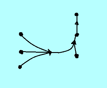they directed, undirected, simple, non-simple,..etc. That's great and graphs are my favorite, but for this post I thought that I'd shake things up a bit...talk about something similar but wacky at the same time ya know? Any guesses? ;-D Well if you read the title of this post it probably won't take you that long to figure it out. This post will be about the less studied but more generalized graph theoretic concept of hypergraphs.

Now I had heard of hypergraphs before, but until now I hadn't set aside enough time to really study them. What I picked up from my brief skimmings of the hypergraph literature was that the edges in hypergraphs could connect more than 3 vertices (in contrast to the graphs that we know where edges are associated with just two vertices). The idea sounded pretty abstract and different to me. No inkling of an idea as to their applications in pure or applied mathematics. To my surprise then when I found out very recently that hypergraphs are being used to store database information. 

WHAAAAAAAAAAAAAAAAAAAAAAAAAAATTTTTT???!!!! :-O

I know I know. You're probably all about as surprised as I was and no doubt itching to read on about the database business. To be as thorough as possible though and to really appreciate the ideas behind the application, let us first look at a more formal definition of hypergraphs and extend that notion to directed hypergraphs. My previous blurb about a hypergraph having "longer" edges will simply not do. 

A graph as I'm sure most of you know, is often defined in more formal terms as a pair of sets V (for the vertices) and E (for the edges). Hypergraphs are also defined in terms of two sets. These can also be denoted as V and E for the vertices and edges respectively. The vertices of a hypergraph are like the vertices of regular graphs; nothing unusual there. The edges though are defined to be non-empty subsets of the vertex sets. If all of the edges in the hypergraph are sets of cardinality two, then we have the regular graphs that we are used to dealing with. Note though that graphs are just special cases of hypergraphs. Following the above definition it is possible to have hypergraph edges that consist of 3 or more distinct elements of the vertex set. 

A natural thought that may creep into your mind is, how are hypergraphs visualized? From what I have seen I don't think that that area of graph visualization has been studied very much (at least relative to the visualization of regular graphs). So far I have only seen two ways of visualizing hypergraphs. The first way simply draws a line or tree connecting the vertices of an edge and assigns an edge labeling to make it clear that the edge covers 3 or more vertices rather than two. The other way that I have seen hypergraphs drawn is by visualizing the vertices of an edge all within some colored blob (being real technical here). Seeing two edges intersect within such a drawing is similar to seeing two sets of a Venn Diagram intersect. 

With the basic idea of a hypergraph in mind let us now see how things like paths and cycles can be generalized in the hypergraph sense. A walk of length k in a hypergraph is defined to be a sequence of k vertices v1 v2,...., vk where vi and vi+1 are contained in a common edge. A path in a hypergraph is then defined to be such a walk in which all of the vertices and edges are distinct. In a closed walk the beginning and ending vertices are the same, and likewise a closed path is a path where the starting and ending vertices match. If any of these definitions sound odd to you just remind yourself about the simplest case in which the hypergraph is a regular graph. Looking at things that way helps to give a more set theoretic view of the graphs that we are used to dealing with. 

The last (or on second thought second to last) generalized graph concept that I thought I would touch up on before getting to the fun database application is the extended hypergraph notion of subgraphs. Remember that subgraphs are basically graphs contained within graphs. They consist of pairs of sets V' and E' where V' and E' are both subsets of the original graphs vertex and edge sets V and E. The definition of a sub-hypergraph is a little bit more involved. Let J = {1,2,...,k} be an indexing set for a subset of hypergraph edges E1, E2,...Ek. Also, let V' be a subset of the hypergraph's vertices. The sub hypergraph induced by V' and J is defined to be the set of intersections between each Ej and V' where the Ej's range from 1 to k and the intersections considered are the nonempty ones. Again it's good to step back from this more abstract notion of subgraphs and think about how this relates to the simpler graph case. In that scenario imagine that the indexing set J goes from 1 to m for all of the m edges in the graph. The above definition then boils down to finding the resulting graph in which the only edges considered are the ones that have endpoints in the vertex subset V'. 

The final notes to make (before moving onto applications) which is really important for this post is the following. Just as hypergraphs generalize the idea of graphs, hypergraphs can also be generalized a bit. How? Well, rather than just pointing to nodes (and again it's assumed that hyperedges can correspond to 3 or more nodes) hyperedges in a more generalized view can "point" to other edges as well. This is the approach that is taken by the database application that we will now touch on. 

This database application is called HyperGraphDB. What it is is an embedded database that uses a hypergraph as its underlying storage mechanism. The nodes and edges (or links as HyperGraphDB calls them) are all categorized as "atoms" of the database (atoms are basically just database entities/objects). The links can of course point to any number of atoms, consistent with the general definition of a hypergraph. The particular example that I have shown here (as bolded code line below) makes use of HyperGraphDB's HGValueLinkg class. There are several link classes defined within HyperGraphDB, HGValueLink being the one you use when you want to associate some sort of value (can be any kind of object) with your hyperedge. In this example I represent my name with a String and pass it as the first argument to the HGValueLink constructor. What comes after that is an array named nodes. Not surprisingly, this array holds information relating to the nodes (and/or links) that are to be contained within the link variable hyperedge. 

HGValueLink hyperedge = new HGValueLink("Tanya", nodes);

Now some of you may be wondering, what exactly is the nodes array? What kind of information does it hold? It turns out that the array does not hold regular object references to the nodes being "connected", but rather to their associated "HGHandle"s. HGHandle is another class defined within the core api. They serve as identifiers for the objects added to the database. For the most part (there are exceptions to this) you will need to refer to an object's handle if you want to do something with it. This is definitely the case when your desire is to remove a node or link from the database. There are times when you can still refer to an atom through it's Java object reference, but from what I've seen so far HyperGraphDB is different in that it emphasizes the use of these handles rather than the traditional approach of using object references to get to things. 

The list of HyperGraphDB's capabilities goes on and on, but I will stop here as the main point of this post was to name a hypergraph database application and show how it conforms to the hypergraph definitions explained earlier. One thing you may still be wondering is, why would someone ever want to use a hypergraph database? What are they good at modeling? The answer depends on what type of data you are looking at and the information that you aim to get out of your data. One of the simplest examples that I could think of is the following. Suppose that you wish to model some of your Google+ hangouts data as a graph. You and all of the people that you have hung out with are the nodes of a graph, and an edge exists between two nodes if the corresponding people hung out. Even if you and two of you hangout buddies all form a cycle, there is no way of telling from this very basic graph model if let's say 3 of you were in a hangout all at the same time. To do that you may have to add information to the nodes and/or edges, partition your vertices into two groups where one of the groups represents people and the other a hangout on a given day or time, or as this post would suggest, model your hangouts in hypergraph style. All of the people involved in the same hangout will be contained within the same hyperedge. This underscores the extreme flexibility of hypergraphs in one sense, but also shows how the best solution can really depend on the problem at hand and what you hope to accomplish. 

If anyone has worked with HyperGraphDB or just hypergraphs as models in general please leave a comment. I am eager to learn more about hypergraphs! :-D

Pig Day and Yellow Pig Day :=)

In case you didn't know, March 1st was Pig Day, one of the lesser known national holidays here in the U.S. of A. I like to quietly celebrate this day by sending out lots of pig pictures to friends via email. Oink! :=) Now even if pigs had absolutely nothing to do with math I would still be tempted to make a posting for them. Why? They are wonderful, intelligent and multitalented creatures. Just do a generic google search on pig intelligence or go looking for them on youtube. In the latter case you'll eventually (if not immediately) stumble upon videos of pigs shaking hands, playing soccer, bowing,singing,..etc. In fact, I've often heard that those who keep pigs as pets have to make sure to keep them mentally occupied. They're smart creatures and are always looking for new things to discover and challenge their minds with.

As it so happens though, pigs do have something to do with math apart from performing calculations for audiences. The link comes through another holiday, Yellow Pigs Day! (celebrated July 17th. What do people do on this day? They eat yellow cake, exchange yellow pig gifts, sing songs and carols about yellow pigs, and think of properties of the number 17. That's an odd sounding festivities list, but with a little background information it will make a bit more sense. I am not sure when Yellow Pig Day was added to the holidays list, but its yellow pig origins can be traced back to the 1960's. Whichever year it actually was, two math students, Mike Spivak and David C. Kelly, were given the assignment of analyzing properties of the number 17. After spending some time mulling over the problem (mind you that 17 has many interesting properties), the two began to joke about a mythical yellow pig with 17 legs, 17 eyelashes (can't remember if it was on each eye or combined...), etc. From that period of hard work and yellow pig musings eventually evolved what we now celebrate as Yellow Pigs Day.

So that explains where the yellow pigs and 17's come from! Interesting huh? :-) This post would not be complete though without mentioning at least one property of 17. I have seen many long extensive lists of the properties of 17 (e.g. its arithmetic properties, its occurrence in architecture, its appearance in important dates and events,..etc.), but what I have not seen much of are the properties of 17 that relate to graph theory. In fact, I have only come across a few. The one that I will discuss here has to do with what are called Ramsey numbers. 

It turns out that there is a whole area of combinatorics research referred to as Ramsey theory. One subcategory of Ramsey theory involves the aforementioned Ramsey numbers which in turn relate to colorings and cliques of complete graphs. At the most basic level this kind of problem can be stated in the following way: 

What is the minimum number R(r,b) such that all complete graphs on R(r,b) vertices with edges colored red or blue contain a complete subgraph of r vertices with all red edges, or a complete subgraph of b vertices with all blue edges. The number R(r,b) is a Ramsey number.It has been proven that such a number exists.

The definition may at first be a little confusing, so the best way to understand it is by considering the following classic problem: show that at a party of 6 people there are 3 who all know each other or three who all don't know each other. Rephrased in graph theory terms the problem boils down to showing that any blue-red edge coloring of the complete graph K6 contains either a 3 cycle of blue edges (Remember that a 3-cycle is K3) or a 3 cycle of all red edges. This interesting factoid can be verified pretty quickly by experimenting a little with edge colorings on K6. As it also turns out, K6 is the minimum complete graph that satisfies this. Trying the same thing out on K5, K4, K3, K2 and K1 will yield nada. To again state things in graph theory lingo, this means that 6 is equal to the Ramsey number R(3, 3). 

This idea of having a minimum number associated with 2 colorings and monochromatic subgraphs can be extended to three or more finite colors. In particular suppose that you have c colors and c integers n1, n2,...nc. The extended result says that there is a complete graph on R(n1,..,nc) vertices and c colors such that for some i between 1 and c there is a complete monochromatic subgraph of color i. The smallest number R(n1,...,nc) that satisfies this property for integers n1,..,nc and c colors is the associated multicolor Ramsey number. 

And that my graphsters and graphistas is all of the background that you will need to understand this post. Phew! Let me now state a very special graph property involving the number 17. Ready.....(drum roll). Wait for it....and...Now! 

R(3, 3, 3) = 17. 

Virtual applause. :-D  

As with all of the things that I write about I like to find out whenever I can when something was proven and by whom. I did a little bit of searching for the information behind R(3,3,3), and after some snooping through the internet found that the multicolor Ramsey number R(3,3,3) was originally found by Greenwood and Gleason in 1955. In addition to the result, what really strikes me as amazing is the way in which it was proven. Evidently Greenwood and Gleason used finite fields to prove their result. Finite fields and graph theory are not two subjects that I would immediately associate with each other. An unexpected surprise. Awesome!!!! :-D 

P.S. Oink!