Tuesday, September 15, 2015

Getting Reacquainted with D3.js

If you don't know, d3.js (the 3 d's standing for Data Driven Documents), is one of the hottest JavaScript data visualization libraries out there. It's extremely popular and many dataviz and general computer science jobs often list it under their lists of desired skills. 

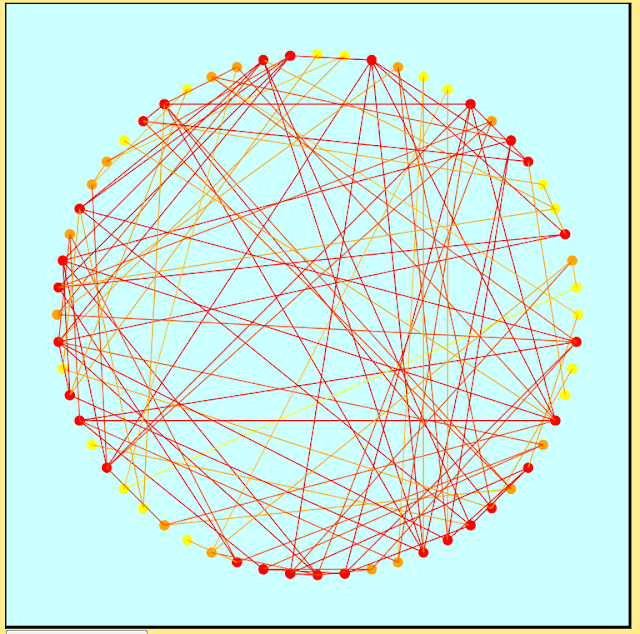
I've used d3 in the past for visualizing graph data, one example being the following circle-based graph layout. Rather than using the traditional black for nodes and edges I decided on a red, orange and yellow color scheme to focus attention to the denser regions of the graph and to reduce visual clutter. The nodes were colored according to degree on a scale ranging from yellow (low degree) to red (high degree). Edges were assigned linear combinations of their endpoints' colors. 


Rather than getting bogged down with all of the color and graph details, I'm going to illustrate some of the basics of d3 using a much simpler example: drawing a grid. The following code accomplishes the task, which I will then explain in subsequent paragraphs. Note that I'm including the surrounding HTMTL code as well. 
____________________________________________________________________

<html> 
<script src = "http://d3js.org/d3.v3.min.js"></script>  
<body> 

<script> 
//create svg element and append to document 
var width = 500; 
var height = 500; 
var svg = d3.select("body").append("svg").attr("width", width).attr("height", height); 

//function for drawing an n by m grid within the svg container 
function create_grid(n, m){ 
  //first draw a rectangle in the svg 
  var rect = svg.append("rect").attr("width", width).attr("height", height)
  .attr("fill", "white").attr("stroke", "black").attr("stroke-width", 3); 

  //draw n-1 horizontal lines and m-1 vertical lines 
  //calculate horizontal and vertical spacings between consecutive lines 
  horizontal_spacing = width/m 
  vertical_spacing = height/n

  for (i = 1; i < n; i++){ 
    svg.append("line").attr("x1",(vertical_spacing)*i).attr("y1", 0)
    .attr("x2", (vertical_spacing)*i).attr("y2", height)
    .attr("stroke", "black").attr("stroke-width", 2); 
  } 

  for (i = 1; i < m; i++){ 
    svg.append("line").attr("x1", 0).attr("y1", (horizontal_spacing)*i).attr("x2", width)
    .attr("y2", (horizontal_spacing)*i).attr("stroke", "black").attr("stroke-width", 2); 
  } 
//create 10 by 10 grid 
create_grid(10, 10); 
</script> 

</body> 
</html> 
____________________________________________________________________

 So the first thing to note before you begin anything is the proper referencing of your d3 library. One option is downloading d3 onto your computer and referencing it, though one can also simply reference the library from online by using src= "http://d3js.org/d3.v3.min.js". There is also a d3.v3.js that one can reference, the difference between d3.v3 and d3.v3.min being that the latter is a more compressed version of the former which is good if speed is your concern. 

Once you have referenced the d3 library you will then want to create your svg element. This will serve as the container element for all of the shapes that you subsequently draw (e.g. rectangles, lines and circles). To do this you will call the select method of d3 to select the body element to which you want to add your svg container. You will then want to append your element of type "svg", and then subsequently set all of the svg attributes such as height and width through the attr method. 

var width = 500; 
var height = 500; 
var svg = d3.select("body").append("svg").attr("width", width).attr("height", height);

Moving along in the creation of what will ultimately be a grid drawing, I decided to create a function called create_grid(n, m) to which you can pass along arguments indicating the number of rows and columns of your grid. That way if you'd like to experiment with other grid sizes you can simply vary the parameters. 

Regardless of your grid dimensions, the first step that you will subsequently want to take is to draw a rectangle within your svg container. Since we already created a variable reference to our svg element, we can simply call the append method onto that, specifying a shape type of "rect" for rectangle followed by the setting of its attribute values, which like the svg, also include things like width and height. Note that I also set attribute values for stroke, stroke-width, and fill. stroke and stroke-width are optional attributes indicating the color and line thickness for the border that is traced out by the rectangle. fill is also optional and is used to indicate the interior color of the rectangle. I chose white for my grid, but one can just as easily create red or pink rectangles by using "red" or "pink" in place of "white". 

 var rect = svg.append("rect").attr("width", width).attr("height", height)
  .attr("fill", "white").attr("stroke", "black").attr("stroke-width", 3); 

The remaining steps involve drawing the vertical and horizontal grid lines according to the specified dimensions. Given inputs of n and m for an n by m grid, this means that we will need to draw n-1 horizontal lines and m-1 vertical lines, which can be accomplished with the following two for loops. I used the horizontal and vertical spacing variables to adjust the spacing between adjacent vertical and horizontal lines respectively, given the fixed svg dimensions. 

  horizontal_spacing = width/m 
  vertical_spacing = height/n

  for (i = 1; i < n; i++){ 
    svg.append("line").attr("x1",(vertical_spacing)*i).attr("y1", 0)
    .attr("x2", (vertical_spacing)*i).attr("y2", height)
    .attr("stroke", "black").attr("stroke-width", 2); 
  } 

  for (i = 1; i < m; i++){ 
    svg.append("line").attr("x1", 0).attr("y1", (horizontal_spacing)*i).attr("x2", width)
    .attr("y2", (horizontal_spacing)*i).attr("stroke", "black").attr("stroke-width", 2); 
  } 

The last and final step: calling the function to create and render the grid within the browser. I chose to create a 10 by 10 grid so my call to the function will be create_grid(10, 10). You will see a result like the following when you open the corresponding html file in a browser. I'm not sure if d3 will load in Google Chrome, and I'm pretty sure that it does not work in Internet Explorer, so to generate my grid drawing I used Firefox. 


And there you have it! A few d3 and JavaScript basics. There are many more aspects to d3 that I haven't covered here, one of the most important being the binding of svg elements to data. Since I was working with a small simple example I thought it would be good to leave that stuff out till  perhaps a future tutorial. For now just have fun playing around with the code and maybe trying to experiment with other shapes and colors. :-) 

Monday, September 14, 2015

Data Visualization Project: The Great Pyramid Builders

I have found sometimes through past experience that rather than drawing tree data (e.g. family trees) according to conventional graph drawing practices or even much fancier and specialized tree drawing algorithms, it can pay to render it in a more list-like tabular form. Featured in this blog post is one such example. It is a visualiation of ancient Egyptian family tree data from the time range of the so-called great pyramid builders. This time period included construction of such famous monuments as the Great Pyramid of Giza, the Pyramid of Khufu and the Bent Pyramid. My motivation for the dataviz project came from a visualization of the same data from The Complete Royal Families of Ancient Egypt, a book which provides data and detailed information on the royal families throughout ancient Egyptian history. My goal was to make a visualization that could incorporate all of the detailed graph data in a way that would be easy for the viewer to trace and follow. 

My initial visualization attempts were aimed at rendering the data in a classic hierarchical fashion. However given the other things that i wished to include such as a timeline and pictures, not to mention the large umber and variety and type of relations (e.g. wife, daughter and son relations along with associated likelihoods), I found the traditional graph drawing route to be too cluttered and complicated. 


That ultimately led me to a major redesign, resulting in the final visualization below which I am quite happy with. The column-like format of the family tree data is much more compact allowing for extra space to be allocated to the pyramid pictures. The tabularized data also matches well with the vertical timeline at left. 

As for how to read the visualization, one can start by looking at the timeline tick marks. These marks run along the timeline and indicate the beginning and ending years of pharaohs' reigns, with rulers running down the central column marked by their cartouches (these are the oval shaped drawings with pharaoh names spelled out in heiroglyphs). Corresponding wives are listed to the left and daughters and sons to the right. I used brown and black lettering for names to distinguish the males from females. It should be noted that due to things such as gaps or inconsistencies in the records, not all relationships can be concluded with certainty. This leads to two additional relationship types indicated at the bottom. The one with the question mark is for uncertain relations between pharaohs and wives/daughters/sons, while the dashed line is for marking an uncertain line of descent between chronological pharaohs. And.... that's about it I think! Pretty cool huh? ^c^ 


NOTE: If you would like to view larger versions of these visualizations with close-up detail you can do so on my dataviz google+ collection: https://plus.google.com/u/0/collection/kg9Bm

Saturday, March 14, 2015

Drawing Bipartite Graphs: A Mutation-Based Approach

Given the popularity of my recent post on genetic algorithm (GA) basics and bipartite graph drawing applications, I decided to summarize another related article here. The paper, "An Experimental Comparison Between Evolutionary Algorithm and Barycenter Heuristic for the Bipartite Drawing Problem" by Zoheir Ezziane, not only presents a GA that compares favorably to the popular barycenter heuristic, but also highlights a topic that is often debated over: the need for a crossover operation in a genetic algorithm. 

Although genetic algorithms can greatly reduce search in the solution space for a problem, they also have the drawback of suffering from typically long computation times. The total computation time can be influenced by many different factors, such as sensitivity to GA parameters(e.g. mutation rate and population size), complexity of the evaluation function, or complexity of the crossover operation. Zoheir makes the same point in his paper. Based on experimental results on bipartite graphs from other papers (listed below), he designs a purely mutation-based GA for bipartite graph drawing (i.e. it has no crossover operation). Unlike the GA from my previous post which fixes the nodes of one of the layers and permutes those of the other, this algorithm rearranges nodes in both layers of the bipartite graph. The algorithm also differs from that described previously in that it does not require the two vertex subsets to be of equal size. 

Thus, assume that we are given a bipartite graph G with vertex sets 1 and 2 of sizes n1 and n2 respectively. The components of Zoheir's genetic algorithm are as follows: 

1. Chromosome representation: Each bipartite graph drawing is represented by two arrays of sizes n1 and n2. These hold the vertices of sets 1 and 2 respectively, and 

2. Evaluation function: The fitness of an individual is equal to the number of edge crossings in the graph drawing induced by its ordering of vertices in layers 1 and 2. 

3. Mutation Operation: This operation has three subparts. 
a. Each vertex v in set 1 mutates with a probability p to another vertex k in the range [1...n1] which has not been selected before. 

b. Each vertex v in set 2 mutates with a probability p to another vertex l in the range [1...n2] which has not been previously selected. 

c. After the mutation operator has been applied to all vertices, reevaluate the number of edge crossings (i.e. the fitness value). 


Parts a. and b. are the same operation applied to different vertex sets, so without loss of generality let's look at an example on the first vertex set of a graph. Suppose for instance that set 1 = {1,3,7,8} and that it's initial ordering within the associated array is [3,7,8,1]. Now let's apply mutations of part a. to the elements of the first set one by one, assuming a mutation rate of p = 0.6. 

1. Take element 1 and suppose that mutation is triggered at that node. We now randomly select some number k from [1...4] (here n1 = 4). Suppose that k = 2. The node located at position 2 of the array 7. 7 has not been selected before, so therefore we swap nodes 1 and 7, creating the new array [3,1,8,7] as a representation of set 1.  


2. Take element 3 and suppose that chance favors mutation here as well. We randomly select k from [1...4] and chance also has it that k = 2. The node located at location 2 of the array is now 1, but 1 has previously been selected/handled by the first step. We must therefore continue to generate random k's until we find corresponding to an array position containing a node that hasn't previously been handled. Let's say that at our second go k = 4. Node 7 is now located at position 4, and it hasn't been previously selected. We thus swap nodes 3 and 7 in the array, creating the new representation [7,1,8,3]. 

3. Take element 7, but suppose that probabilities are not in our favor this time and we skip a mutation step. The array then remains as it was at the end of step 2 as [7,1,8,3]. 

4. Take element 8 and suppose that mutation is triggered at that node. We randomly generate k which comes out to 3. The node located at position 3 is 8 itself. We therefore leave 8 alone and have [7,1,8,3] as our final array representation for vertex set 1. 

4. Selection Policy: Following a random generation of an initial population P0, individuals are created through crossover and mutation applied to pairs from P0 until the total number of new individuals is equal to the size of P0. An elitist selection policy is then applied in the following way. Take the best (i.e. the fittest) member of P0 and the best of the current population. If the best member of the current population is less fit than the best member of the previous, replace the worst member of the current population with the best of the previous. If, on the other hand, the best member of the current population is more fit than that of the previous generation, then leave the current population alone. This current population will then be taken as the new generation to be evaluated for subsequent iterations of the GA. After each new generation of individuals is created through crossover and mutation the selection policy will perform any replacements deemed necessary by the described elitist method. 

And there you have it, what I would consider to be the bulk of the genetic algorithm. :-) What remains to explain now are the specific parameters used by Zoheir and the results he found when comparing the algorithm to the barycenter heuristic. 

A mutation rate (the probability p used in the mutate operation) or 0.8 was used throughout the simulations. Also, the total size or order of a bipartite graph was considered rather than the sizes of the individual vertex subsets. So in his analysis a graph of order 6 could have vertex subsets of sizes 5 and 1, 2 and 4, or 3 and 3. 


An important graph metric considered throughout the simulations was that of graph density. In the context of a bipartite graph having vertex subsets of sizes m and n, the graph density is defined to be the ratio |E|/(m*n). |E| denotes the cardinality of its edge set. 

The following list includes some of the highlights of the simulated results: 

1. Starting with a small population size of 10 and assuming a bipartite graph of order 10, the GA always outperformed the barycenter heuristic regardless of density. The trade off here comes in terms of time. It was found that the total number of iterations needed to outperform the barycenter heuristic in this scenario reached 200. 

2. Not surprisingly with a larger population size of say 30, fewer iterations were needed to surpass the results of the one-sided barycenter heuristic. The total number of iterations needed for the GA to do so never exceeded 50 in this case due to the variety of solutions offered by the larger population size. 

3. The GA always eventually outperforms the barycenter heuristic on graphs with density greater than 50%. 

4. The GA always eventually outperforms the barycenter heuristic on graphs with density less than 50%, but with generally larger population sizes (specific population numbers are graphed in the results section). 

5. On graphs of order 17 the average number of iterations needed by the GA varied dramatically based on the density of the graph. 

So to summarize, what we can take away from all of this is that a purely mutation-based genetic algorithm also shows successful performance in drawing bipartite graphs. When tested on bipartite graphs of orders 10 and 17, it was found to eventually outperform the classical barycenter heuristic in terms of edge crossing minimization. The trade off came in terms of time, with the total number of iterations needed to exceed the barycenter result reaching a maximum of 200. If the ultimate goal is to have the cleanest possible graph drawing with the fewest number of edge crossings, or if one is dealing with bipartite graphs that are pretty small in size, then this is not that big of a sacrifice. 

Another interesting result to take out of this study is the finding that the number of iterations of the GA varied quite a bit with graph density. This highlights the importance of considering graph density, rather than graph size alone, as a complexity measurement in these types of graph drawing studies. 

References: 
1. Ezziane, Z. 2007. Experimental Comparison Between Evolutionary Algorithm and Barycenter Heuristic for the Bipartite Drawing Problem. J. Comput. Sci., 3: 717-722. 

2.  Newton, M., O. Sykora, M. Withall and I. Vrto, 2002. A PVM Computation of Bipartite Graph Drawings. http://parc.lboro.ac.uk/research/projects/parseqgd/s topara/stopara.pdf accessed on 6th August 2006. 

3. Rosete-Suarez, A., M. Sebag and A. OchoaRodriguez, 1999. A study of Evolutionary Graph Drawing. Technical Report, http://citeseer.ist.psu.edu/411217.html accessed on 7th November 2006. 

4. Branke, J., F. Bucher and H. Schmeck, 1997. A Genetic Algorithm for Undirected Graphs. In J. T. Alnader Edn., Proceedings of 3 rd Nordic Workshop on Genetic Algorithms and their Appli., 193-206.


Thursday, March 5, 2015

Genetic Graph Drawing Algorithms: A Bibliography

This is a quick follow up to my previous post about genetic algorithms and a GA for bipartite graph drawing. What follows is a listing (not properly formatted, sorry) of papers I've found on the topic of genetic graph drawing. I included the paper discussed in the previous post as well. This area of graph drawing is pretty new to me, though some some promising areas of application seem to be in the visualization of bipartite graphs and lattice graphs. Apart from specific graph examples the approach also seems appealing in that one can explicitly hard code into the evaluation function things like symmetries, sum of edge lengths, maximum edge lengths,...etc. to be optimized in the graph drawing, essentially tailoring the desired output according to your own visual preferences. This contrasts with other common graph drawing techniques (e.g. spectral and force-directed methods) which model the graph drawing problem in terms of minimizing some energy function which can of course result in optimal values for said aesthetic parameters but don't explicitly make clear which ones will be optimized if any from the get go. For those readers who also find this topic interesting, happy reading! :-)

Genetic Graph Drawing Papers: 


  1. Peter Eades, Hugo A.D. do Nascimento, A Focus and Constraint-Based Genetic Algorithm for Interactive Directed Graph Drawing, The Second International Conference of Hybrid Intelligent Systems, 2002.
  2. Bernadete M.M. Neta, Gustavo H.d. Araujo, Frederico G. Guimaraes, Renato C. Mesquita, Petr Ya. Ekel, A fuzzy genetic algorithm for automatic orthogonal graph drawing, Applied Soft Computing 12, 2012
  3. Brian Loft and John Snow, A Genetic Algorithm for Drawing Ordered Sets, Texas College Mathematics Journal, Volume 3 Issue 2, 2006
  4. Hobbs and Rogers, Representing Space: A Hybrid Genetic Algorithm for Aesthetic Graph Layout
  5. Bernadete M. Mendonca Neta, Gustavo H. D. Araujo, Frederico G. Guimaraes, A Multiobjective Genetic Algorithm for Automatic Orthogonal Graph Drawing, ACM, 2011
  6. Salabat Khan, Mohsin Bilal, Muhammad Sharif, Farrukh Aslam Khan, A Solution to the Bipartite Drawing Problem Using Genetic Algorithm
  7. Rosete-Suarez, M. Sebag, A. Ochoa Rodriguez, A Study of Evolutionary Graph Drawing
  8. Qing-Guo Zhang, Hua-Yong Liu, Wei Zhang, Ya-Jiun Guo, Drawing Undirected Graphs with Genetic Algorithms, ICNC 2005
  9. Dhamyaa A. AL-Nasrawi, Najah A. Rabee, Ausay A. Ja’afar, Karrar I. Mohammed, Evolutionary Algorithm Implementation for Good Graph Drawing Using Fuzzy Fitness Function
  10. Gudenberg, Niederle, Ebner, Eichelberger, Evolutionary Layout of UML Class Diagrams
  11. Toshiyuki Masui, Evolutionary Learning of Graph Layout Constraints from Examples, Proceedings of the ACM Symposium on User Interface Software and Technology, 1994, ACM Press, pp 103-108
  12. Zoheir Ezziane, Experimental Comparison Between Evolutionary Algorithm and Barycenter Heuristic for the Bipartite Drawing Problem, Journal of Computer Science 3, Issue 9, 2007
  13. Mohamed A. El-Sayed, GA for straight-line grid drawings of maximal planar graphs, Egyptian Informatics Journal, 2012
  14. Erkki Makinen and Mika Sieranta, Genetic Algorithms for Drawing Bipartite Graphs, Department of Computer Science University of Tampere, Report A-1994-1
  15. Dana Vrajitoru and Boutros R. El-Gamil, Genetic Algorithms for Graph Layouts with Geometric Constraints
  16. HE, H., Sykora, O. and Makinen, E., 2007. Genetic Algorithms for the 2-page book drawing problem of graphs, Journal of Heuristics, 13 (1), pp. 77-93
  17. Behrooz Koohestani, Genetic Hyper-Heuristics for Graph Layout Problems, PhD Thesis, Department of Computer Science University of Essex, 2013
  18. Dana Vrajitoru, Multiobjective Genetic Algorithm for a Graph Drawing Problem
  19. Timo Eloranta and Erkki Makinen, TimGA: A Genetic Algorithm for Drawing Undirected Graphs, Divulgaciones Matematicas Vol. 9, No. 2, 2001, pp. 155-171
  20. Jiayu Zhou, Youfang Lin, Xi Wang, Visualization of Large-Scale Weighted Clustered Graph: A Genetic Approach, Proceedings of the Twenty-Third AAI Conference on Artificial Intelligence, 2006

Wednesday, March 4, 2015

Drawing Bipartite Graphs: A Genetic Algorithmic Approach

It was somewhat recently in a course I'm taking that the basics

of so-called genetic algorithms were discussed. These "genetic" algorithms are ones that have been designed to mimic the various steps of natural selection. That is, a genetic algorithm (GA for short) consists of the following steps and components.  

1. Initialization: Start the process with some initial population, call it P0. The fitness of each individual in P0 is measured by some fitness evaluation function.  

2. Breeding: From P0 pairs of individuals are selected (usually with some probability relevant to their fitness values), to breed and produce offspring for the next generation. 

3. Genetic Operators: During the breeding phase of the algorithm,genetic material from selected parents undergo crossover and mutation operations. The crossover operation combines portions of the parent's genetic material into one genome, and mutation then randomly changes portions of it. The final result is the genome of a child from the pair. 

4. Selection: Following the breeding of pairs from P0, the fitness values of all individuals (children and parents) are evaluated for selection for the next generation. Typically the ones with the highest fitness values are chosen, with some selection rules also dictating that portions of the previous population also be included in subsequent iterations of the algorithm. 

Following the selection of a new (and hopefully fitter) population in step 4, steps 2 through 4 are repeated until some termination condition is reached (e.g. some predefined number of steps has passed or the average population fitness has stabilized). 

So that is the basic outline of a genetic algorithm. Why am I talking about all of this here? Well apart from it being inherently interesting I was amazed to hear that the approach has been applied to areas of graph drawing. :-0 (that was my face when I found that out). I'm always excited to learn about new graph drawing algorithms and even more so new areas of graph drawing, so you can probably imagine I was pretty stoked about all of this. Researching the topic a little bit more I discovered that quite a few articles had been written about it, with algorithms designed for drawing undirected, orthogonal, directed, bipartite, and lattice graphs. I'm still in the process of skimming over all of the articles I found, though one area of genetic graph drawing that appears promising to me is in the drawing of bipartite graphs. For the remainder of this post I've decided to summarize one such algorithm by Makinen and Sieranta from their article "Genetic Algorithms for Drawing Bipartite Graphs". It's very interesting and will also give a better idea through example of what genetic algorithms are like. 

Bipartite graphs are traditionally drawn in a layered fashion, with each vertex subset assigned to its own (usually horizontal) layer. Since the layers determine the y coordinates of the graph's nodes beforehand, what remains is to assign x coordinates to the vertices in a way that makes the drawing as clear as possible, typically by minimizing the number of edge crossings. One key observation relating to this is the fact that the number of edge crossings in a bipartite graph drawing depends on the ordering of nodes within layers rather than on the actual assigned x coordinates. Thus the problem of drawing bipartite graphs reduces to a permutation problem of nodes within layers that minimizes edge crossings. Vertices can be permuted in both layers to achieve this, though some algorithms take the alternative approach of fixing  the x coordinates in one layer and permuting the vertices in the other layer (referred to as the level permutation problem or the one sided crossing minimization problem). Both approaches to permuting layers to minimize edge crossings turn out to be NP-Hard, so heuristics are required to approximate solutions to them. Makinen and Sieranta take the approach of permuting a single layer in their algorithm. 

Makinen and Sieranta assume at the beginning that their graphs have equal sized vertex subsets.That is, given a bipartite graph G  with disjoint vertex sets V1 and V2, it is assumed throughout their paper that |V1| = |V2| = n. Here n is some positive integer called the size of the graph. The maximum number of edges that can occur in such a graph of size n is n*n = n^2. Letting E denote the edge set of G the authors define the edge density of G to be |E|/(n^2). What follows now are the key components to their genetic algorithm.  

1. Chromosome representation: Each individual is represented as a permutation of the numbers 1 through n, indicating an ordering of the graph's nodes within the layer that is to be rearranged. So for example suppose that the graph size is 3 and that the vertices of V2 = {v1, v2, v3} are to be permuted. A permutation written as (3,1,2) means that v3 has an x coordinate of 1, v1 an x coordinate of 2, and v2 an x coordinate of 3 (i.e. 3 goes to 1, 1 goes to 2, and 2 goes to 3).

2. Evaluation Function: the fitness of an individual is evaluated as its total number of edge crossings in the corresponding bipartite graph drawing. The desire is to have a drawing with fewer edge crossings and less clutter, so a permutation of the non-fixed layer is considered more fit in this context if it induces fewer edge crossings. 

3. Population Size: Through experiment (details omitted here) the authors found an optimal population size of 50. It is important to choose a good population size since one that is too small may not be representative of the space of potential solutions while one that is too large can hinder the search process of the algorithm. 

4. Crossover Operation: This operation takes two individuals x and y with permutations x = (x1, x2,...,xn) and y = (y1, y2,...,yn), and uses them to produce two new offspring. First, two random integers i and j with i < j are generated from the range [1...n]. Next the segments xi,...,xj and yi,...yj are retrieved from each parent. Each segment occupies positions i through j in the permutations of the generated children. The remaining permutation positions are augmented by numbers from the set {1,...,n} that haven't yet been included. They are listed in the order that they appear in the other parent. So for instance the child that has a segment from x is augmented by the remaining positive integers in the order that they appear from left to right in y. 

The authors illustrate this operation through the following example. Suppose that our parents are x = (1,2,3,4,5,6) and y = (2,4,5,1,6,3). Also assume that we have generated the random integers i = 3 and j = 5. Our x and y segments will be (3,4,5) and (5,1,6) respectively. The augmented x segment will become (2,1,3,4,5,6). The other child will be (2,3,5,1,6,4). 

5. Mutation Operation: Suppose that we are given a permutation x = (x1,x2,...,xn). For each xi a random real number r from [0...1] is generated and compared to some fixed mutation rate, call it r'. If r < r', then a mutation will proceed as follows. Suppose that we have generated a random real r that is less than r' for xi. Generate a random integer j from [1...n]. If i < j then move xi to position xj and shift all elements xk where k = i+1,...,j one position to the left. If i > j then move xi to the position of xj and shift all all elements xk with k = j,...,i-1 one position to the right. The authors suggest using a mutation rate of r' = 0.03 (derivation details omitted here). 

6. Selection Policy: The authors found the following selection/breeding policy to be the most helpful (here they are combining the two genetic algorithm steps into one). First, pick the fittest individual in the current population (this requires counting the number of edge crossings in all of the induced bipartite drawings). This individual will be included in the next generation. For the remainder of the population, create two subpopulations A and B. A (respectively B) consists of individuals with a crossing number that is below (respectively above) the average crossing number of the whole population. Randomly select one parent from A, one from B, and apply crossover and mutation to produce two children for the next generation. Repeat this step on sets A and B until a new population size of 50 is created. 

Thus the algorithm of Makinen and Sieranta begins with an initial population P0 of permutations (all corresponding to the same layer that is to be rearranged for the graph drawing), and applies the selection/breeding policy to produce a new population P1. This policy is again applied to P1, and continues iteratively until some termination condition is reached. Going through the paper I didn't see any fixed termination condition; it seemed to vary according to the graph size. For smaller graphs of size 15 (remember that this means 15 nodes in each layer) it appears that they terminated their genetic algorithm after a little over 60 iterations. For larger graphs of size 20 and 30 they specified using at least 100 generations (i.e. iterations of the algorithm), and stopping after 50 consecutive generations showed no improvements in terms of edge crossings. 

The authors did find favorable results with their algorithm. They compared their results to the classical barycenter heuristic (BC for short), which handles one sided permutation by moving a node in say V2 (the layer to be permuted) to the average x coordinate of its neighbors in V1. Specifically they found the following results: 

1. Comparing best results, they found their GA to perform as much as 2% better than BC on graphs of size 15 with 10% density (i.e. a low density). The results were about the same as BC with higher density (around 50%) size 15 graphs. 

2. For graphs of size 20 and density 30% 100 random bipartite graphs were generated. After running at least 100 iterations of the genetic algorithm until 50 consecutive generations showed no difference in total edge crossings, they found the average difference of their output compared to that generated by BC to be 0.3%. For graphs of size 30 and density 30% the average difference between their GA and BC was 0.5%.

Several comments should be made regarding these results, as some of these numbers may not appear that impressive at first glance. For starters, a graph size of 15, 20 or even 30 might not sound very large, though a lot of the bipartite subgraphs of multi-layered graphs that I've encountered haven't been very large, so if that is representative of bipartite graphs and mult-layered graphs in general then it really isn't such a bad thing that the graphs considered in the study are small.  

Also, a 2% difference in results may not sound very large, let alone differences of 0.5 or 0.3 percent. Remember though that this difference is being taken over the number of edge crossings, which can get quite large as the underlying combinatorics of the bipartite graph become more complicated. Thus even a small percentage difference can correspond to quite a few edge crossings and visually make quite the difference in the graph drawing's appearance. 

So, punchline is that the GA, which was quite simple, did in fact compare favorably to a well known heuristic in one sided crossing minimization. I'm currently studying more applications of genetic algorithms in graph drawing including another GA for drawing bipartite graphs. If I don't write another post that summarizing a genetic graph drawing algorithm I'll at least post a listing of the articles that I've found in the area for interested readers. :-) 


References: 
Genetic Algorithms for Drawing Bipartite Graphs by Erkki Makinen, Mika Sieranta-Intern. J. Computer Math, 1994


Thursday, January 22, 2015

Spectral Graph Drawing: The Basics

Okay so it's been a ridiculously long time since I've posted anything. Yes I still love graphs and of course I still love graph drawing. The latter is what I have, in particular, been focusing on as of late. The particular topic that's been getting my undivided attention is spectral graph drawing. Under this approach the positions of a graph's nodes in 1, 2 or 3 dimensions are determined by the entries of certain eigenvectors of a graph related matrix. Many different matrices can be used for this purpose, though at the most basic level one utilizes the eigenvectors of the so-called Laplacian matrix of a graph. 

For starters what exactly is a graph's Laplacian? Well if one was to define D to be the diagonal matrix with a graph's degree sequence along the main diagonal and A as the typical adjacency matrix of the graph, then the Laplacian L is defined to be the difference L = D-A. It is generally assumed in the literature that the graph being visualized is undirected, and lacks loops and multiple edges. We can assume, however, that the edges of the graph are weighted, though only with nonnegative real numbers. 

Besides its cool name, the Laplacian receives a lot of interest in spectral drawing research because of several desirable properties that it has. I'll summarize these without proofs below as a 'Theorem'. 

Theorem: Let G be a graph on n nodes as described thus far and let L be its Laplacian matrix: 
a. L is symmetric positive semi definite
b. L has eigenvalue 0 with the corresponding eigenvector of all 1's
c. The multiplicity of the eigenvalue 0 is equal to the number of connected components in the graph. 


Positive semi-definite means that if you take any vector x with n entries and calculate the product x*Lx (where x* denotes the transpose of x) then the result will be a nonnegative number. Symmetric means that L and its transpose are the same. There happens to be a very nice result in matrix theory which says that the eigenvalues of a symmetric positive semi-definite matrix are all real and nonnegative. Thus all the eigenvalues of the Laplacian of an undirected graph with nonnegative weights are nonnegative real numbers. The eigenvectors of L also have the nice property that if you take any two eigenvectors xi and xj corresponding to different eigenvalues they will be orthogonal to each other (i.e. the dot product of xi and xj will come out to zero). :-0

Righteous! Okay. So up to this point we've seen something called the Laplacian of a graph and some technical properties of it that are supposedly nice, though things are still looking pretty abstract and the connection to graph drawing is not readily apparent. The thing or rather equation that helps to tie all of these loose strings together is what has come to be called Hall's Energy function. The function is named after Kenneth Hall. He was the first to suggest the utilization of graph spectra for drawing purposes and modeled the problem of visualizing a graph in one dimension by the following set of equations: 
The minimization is of Hall's energy function described in the first line. It is taken over all real n dimensional vectors x. The second equation puts a normalization constraint on the solution to ensure that x has unit norm and the area of the drawing remains compact. The final equation asks that your solution x be orthogonal to the vector of all one's. This is to avoid the trivial solution of placing all nodes on the same position of the real number line. As this suggests the minimizing vector will determine the x coordinates of the graph's nodes. 


To continue with the hand waving, this won't be proved here, but one can also show that the critical points for minimizing the energy of Hall's function are exactly the eigenvectors of L. It's pretty simple to prove using substitution into x*Lx that the resulting output values will be the corresponding eigenvalues. The absolute minimum of the function of course occurs when all xi are equal, but again that would pack all nodes into the same spot and would do nothing for us in terms of revealing information on the graph's structure. The best one can do then is to take the second best solution. This occurs at the eigenvector for the second smallest nonzero eigenvalue, call it x2 (it will be orthogonal to the all one's vector because of the pairwise orthogonality for eigenvectors of symmetric matrices). Turns out it has a very special name: the Fiedler vector ;D 

The above derivation can be generalized to 2, 3 or even k dimensions. For the case of 2 dimensions Hall describes two sets of equations where the second is much like the first from above. The only difference is that instead of a vector x we are looking for another one, call it x3, which satisfies the same constraints as above but is also orthogonal to x2. The result will be the third smallest nonzero eigenvector. x2 and x3 together will give the x and y coordinates of our graph's vertices. 

Phew! That was a lot of setup (mainly because of the underlying theoretical justification). The very nice thing about all of this eigenvector business though is that the graph drawing can be computed quickly and the result is exact and globally optimal. This is in contrast to other graph drawing problems which tend to be very VERY difficult (in the NP Hard class) and which often require inexact heuristics and suboptimal solutions. It also has a natural interpretation. Nodes that are more related to each other and have high edge weight should be placed closer together so that their coordinate differences contribute less to the sum. Those that are less related with smaller edge weights can be placed further apart without increasing the sum by a significant amount. 

This latter point also highlights a potential drawback, however, and that is the tendency of spectral drawings obtained through this method to smoosh clusters of highly related nodes into small spaces of the total drawing area and placing outlier nodes on the outer edges. When presented with a drawing like this it is difficult to make out much of the graph's structure, especially in the highly clustered regions. If all one wants to know is the existence of said clusters and doesn't care much for the finer details then that's all okay, but for those who want to gain a deeper insight into a graph's structure they may need to use more sophisticated spectral techniques. 


I will end it all here for the time being and move on with an example of a spectral graph visualization. The more sophisticated spectral drawing techniques will be reserved in later posts. 

What you see below is a graph visualization obtained using the two smallest nonzero Laplacian eigenvectors for a dolphin social network in New Zealand :-). 62 dolphins in total were recorded and an undirected social network was created to model their frequent associations with each other. Each dolphin was given its own name, but to clean up the visualization I decided to omit them here. The data comes from: D. Lusseau, K. Schneider, O.J. Boisseau, P. Haase, E. Slooten and S.M. Dawson, Behavioral Ecology and Sociobiology 54, 396-405 (2003). The actual visualization was produced by the draw_spectral method in python's networkx module. 

It's clear from the drawing that there are some cliques within the dolphin network. The details of the one at top right are easier to make out and there are some definite outliers with few associations like the ones at bottom right. However, the clique to the top left is much more collapsed and spiked in appearance. To make out the individual associations here better one would need a more sophisticated algorithm, and perhaps one with good zooming in features. These, as I said before, will be the topic of future posts, so if spectral graph drawing floats your boat, stay tuned! :-D